Lorem ipsum dolor sit amet, consectetur adipisicing elit. Odit molestiae mollitia laudantium assumenda nam eaque, excepturi, soluta, perspiciatis cupiditate sapiente, adipisci quaerat odio voluptates consectetur nulla eveniet iure vitae quibusdam? Excepturi aliquam in iure, repellat, fugiat illum voluptate repellendus blanditiis veritatis ducimus ad ipsa quisquam, commodi vel necessitatibus, harum quos a dignissimos.
Close Save changesHelp F1 or ? Previous Page ← + CTRL (Windows) ← + ⌘ (Mac) Next Page → + CTRL (Windows) → + ⌘ (Mac) Search Site CTRL + SHIFT + F (Windows) ⌘ + ⇧ + F (Mac) Close Message ESC
So far, we considered inference to compare two proportions and inference to compare two means. In this section, we will present how to compare two population variances.
Why would we want to compare two population variances? There are many situations, such as in quality control problems, where you may want to choose the process with smaller variability for a variable of interest.
One of the essential steps of a test to compare two population variances is for checking the equal variances assumption if you want to use the pooled variances. Many people use this test as a guide to see if there are any clear violations, much like using the rule of thumb.
When we introduce inference for two parameters before, we started with the sampling distribution. We will not do this here. The details of this test are left out. We will simply present how to use it.
To compare the variances of two quantitative variables, the hypotheses of interest are:
Null AlternativesThe last two alternatives are determined by how you arrange your ratio of the two sample statistics.
We will rely on Minitab to conduct this test for us. Minitab offers three (3) different methods to test equal variances.
Bonett’s test and Levene’s test are both considered nonparametric tests. In our case, since the tests we will be considering are based on a normal distribution, we are expecting to use the F-test. Again, we will need to confirm this by plotting our sample data (i.e., using a probability plot).
Caution! To use the F-test, the samples must come from a normal distribution. The Central Limit Theorem applies to sample means, not to the data. Therefore, if the sample size is large, it does not mean we can assume the data come from a normal distribution.
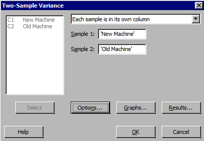
Using the data in the packaging time from our previous discussion on two independent samples, we want to check whether it is reasonable to assume that the two machines have equal population variances.
Recall that the data are given below as (machine.txt):
New Machine| 42.1 | 41.3 | 42.4 | 43.2 | 41.8 |
| 41.0 | 41.8 | 42.8 | 42.3 | 42.7 |
| 42.7 | 43.8 | 42.5 | 43.1 | 44.0 |
| 43.6 | 43.3 | 43.5 | 41.7 | 44.1 |
Notes on using Minitab:
The Minitab Output for the test for equal variances is as follows (a graph is also given in the output that provides confidence intervals and p-value for the test. This is not shown here):
σ1: standard deviation of New machine
σ2: standard deviation of Old machine
F method was used. This method is accurate for normal data only.
| Variable | N | StDev | Variance | 95% CI for σ |
|---|---|---|---|---|
| New Machine | 10 | 0.683 | 0.467 | (0.470, 1.248) |
| Old Machine | 10 | 0.750 | 0.562 | (0.516, 1.369) |
| Estimated Ratio | 95% CI for Ratio using F |
|---|---|
| 0.911409 | (0454, 1.829) |
| Method | Test Statistic | DF1 | DF2 | P-Value |
|---|---|---|---|---|
| F | 0.83 | 9 | 9 | 0.787 |
Note that \(S_=0.683\) and \(s_=0.750\) The test statistic \(F\) is computed as.
The p-value provided is that for the alternative selected i.e. two-sided. If the alternative were one sided, for example if our alternative in the above example was "ratio less than 1", then the p-value would be half the reported p-value for the two-sided test, or 0.393.
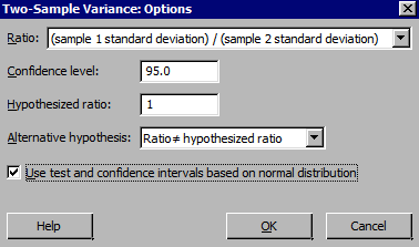
Minitab provided the results only from the F-test since we checked the box to assume normal distribution. Regardless, the hypotheses would be the same for any of the test options and the decision method is the same: if the p-value is less than alpha, we reject the null and conclude the two population variances are not equal. Otherwise, if the p-value is large (i.e. greater than alpha) then we fail to reject the null and can assume the two population variances are equal.
In this example, the p-value for the F-test is very large (larger than 0.1). Therefore, we fail to reject the null hypothesis and conclude that there is not enough evidence to conclude the variances are different.
Note! Remember, if there is doubt about normality, the better choice is to NOT use the F-test. You need to check whether the normal assumption holds before you can use the F-test since the F-test is very sensitive to departure from the normal assumption.